Using Vegetation, Precipitation, and Surface Temperature to Study Climate Zones

Purpose: Explore the relationship between amount of vegetation, precipitation, and surface temperature to study Earth's climate zones.
Estimated Time for Completing Activity: One 50-minute period
Lesson Links:
- Koeppen (also known as Koppen) Classification System
- Live Access Server (Intermediate Edition)
- Sample NDVI graph
- CERES/SARB Surface Properties
- Normalized Difference Vegetation Index NDVI description
- Convert this Lesson into a PDF
Background:
The type of climate present in a particular location depends on several variables, including surface temperature and annual precipitation. One indicator of a locale' s climate is the vegetation present, a relationship used by the Koeppen system of climate classification. See Lesson Links above for information on that system.
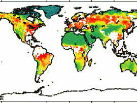
The type and amount of vegetation is one piece of data collected by the Multi Angle Imaging SpectroRadiometer, or MISR, instrument on the Terra satellite. Rather than taking a photograph of the vegetation, the instrument records the type of light, ultraviolet and infrared, reflected from the foliage of the various plants. Scientists then mathematically process the data, and the result is known as the Normalized Difference Vegetative Index, or NDVI.
Scientists are interested in learning how the vegetation of an area can be used to study Earth' s climate. In this activity, the student will make a similar study. For a selected location, the student will investigate possible relationships between the vegetation index, the precipitation, and the surface temperature data over several years' time. Using that information, the student will predict the climate type, and will compare the prediction to a climate classification chart.
Procedure:
Part I. NDVI Plot
1. Click on the Live Access Server (Intermediate Edition) found in the lesson links above.
2. If you are not automatically prompted click on 'Choose Dataset' found at the top left of the page then, click on Life, and then Monthly Normalized Difference Vegetation Index (MISR).
3. From the menu to the left of the screen, select 'Time Series' found under 'Line Plots'.
4. Under the navigation map to the left, in the latitude and longitude boxes, enter 22S and 135E
5. Under Select time range, from the pull-down menu, select Jan 2002 to Jun 2004
6. The graph of NDVI should appear. Either Print or Save the image for later use.
Part II: Surface Temperature Plot
1. Repeat step 1of Part I.
2. This time click on Land, and then Monthly Surface Clear Sky temperature. (ISCCP)
3. Repeat steps 3-6 of Part I.
4. The graph of Surface Temperature should appear. Print or Save for later use.
Part III: Precipitation Plot
1. Repeat step 1of Part I.
2. This time click on Water, and then Monthly Precipitation (GPCP).
3. Repeat steps 3-6 of Part I.
4. The graph of Precipitation should appear. Print or Save for later use.
Part IV: Making graphs for other locations
1. From Parts I-III, you now have three graphs for the same location (22S, 135E): NDVI, Surface Temperature, and Precipitation. Note that gaps in the line plots indicate that data is missing for those dates.
2. Repeat Parts I-III for the following locations: 48N 93 W, 6.5 S 42.2W, 41.2N 81.2W.
3. Print or Save all nine graphs for future use. You now have a total of 12 graphs.
Questions:
1a. For each of the four locations, using the graphs of NDVI, temperature, and precipitation, predict the climate zone: Cold, Temperate, Dry, or Tropical. Record your predictions for each.
1b. Using an atlas and referring to the Koeppen's Climate Classification (See Links section), identify the climate type for each location.
1c. Compare your prediction to the identified climate zone. Discuss the similarities and differences.
2. According to the NDVI information (see Glossary) what types of vegetation would you expect to find in each location?
3. Do you think the NDVI is a good predictor of climate zones? Referring to the graphs, explain your answer.
Extensions:
1a. Identify the city determined by the latitude and longitude of the four locations used in the Procedure.
1b. Using on-line or other resources find the average annual rainfall, elevation, and native vegetation for each of the cities.
1c. Does the information you found support your predicted Climate Zone for each city?
2a. Look at the 12 graphs you have plotted. Do you see any patterns in where or when data is missing?
2b. Using information you have found from reading about ISCCP and MISR (see Glossary), what would cause data to be missing?
3. Using the procedure summarized below, generate a world-wide image of NDVI for June, 2004. Compare this image to the Koeppen map. Do you see any similarities or differences in the patterns between the two images? Repeat for December 2003. Write a summary statement about what you found.
Procedure summary: Follow the steps for Part I of the lesson, except select Longitude-Latitude map (xy), Color plot, and Full Region. (These are the default choices, so they should already appear in the boxes.) For the Time range, use the pulldown menu to choose 2004-06 (June, 2004). Click on Next.
4a. Using the CERES SARB Surface Properties map (see Links section), compare this map to the Koeppen map. What are the similarities or differences between the two maps? Write a summary statement about what you found.
4b. Refer to the CERES SARB Surface Properties map (see Links section). Click on or near the location of one of the cities studied earlier in the lesson. Does the information on surface types agree with the types of vegetation you found in your research? Repeat for each city, then write a summary statement to describe your findings.
Please Contact Us to Receive the Answer Keys
(please note, we can only provide the answer keys for "GPM Original" lesson plans)

